Create and plot boundaryData for DFSEM from a 1D RANS simulation

This example shows how to create a boundary data for turbulentDFSEM inlet boundary condition. In addition, the script also plots the profiles for verification.

First create a 1dprofilDFSEM with create1dprofilDFSEM

from fluidfoam import create1dprofilDFSEM, read1dprofilDFSEM
import os

basepath = "../../output_samples/DFSEM/"

case3d = "3D/"
case1d = "1D/"

sol1d = os.path.join(basepath, case1d)
sol3d = os.path.join(basepath, case3d)

boundary_name = "inlet/"
axis = "Y"

create1dprofilDFSEM(sol1d, sol3d, boundary_name, "200", axis,
                         "U","k","omega","turbulenceProperties:R","Y")
# if turbulenceProperties:R does not exist type:
# "pimpleFoam -postProcess -func R -time 200"
# in a terminal

Y, U, L, R, ny = read1dprofilDFSEM(sol3d, boundary_name, "0", axis)

Reading file ../../output_samples/DFSEM/1D//constant/polyMesh/owner
Reading file ../../output_samples/DFSEM/1D//constant/polyMesh/faces
Reading file ../../output_samples/DFSEM/1D//constant/polyMesh/points
Reading file ../../output_samples/DFSEM/1D//constant/polyMesh/neighbour
Reading file ../../output_samples/DFSEM/1D/200/U
Reading file ../../output_samples/DFSEM/1D/200/k
Reading file ../../output_samples/DFSEM/1D/200/omega
Reading file ../../output_samples/DFSEM/1D/200/turbulenceProperties:R

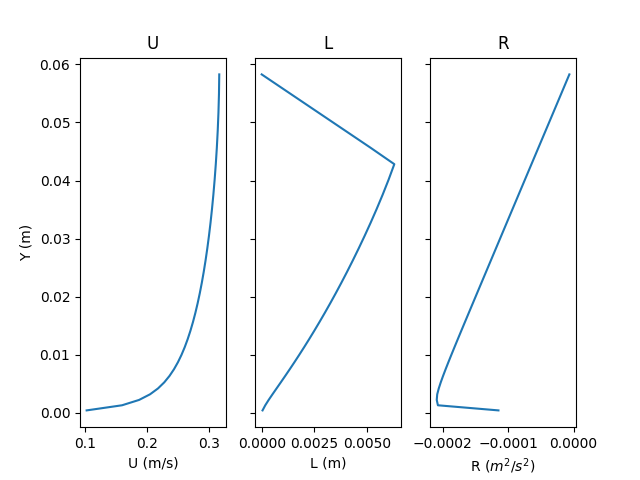
Now plot the profiles of the fields

import matplotlib.pyplot as plt

fig, axarr = plt.subplots(1, 3, sharey=True)
axarr[0].set_ylabel("Y (m)")
axarr[0].plot(U[:], Y)
axarr[0].set_title("U")
axarr[0].set_xlabel("U (m/s)")

axarr[1].plot(L[:], Y)
axarr[1].set_title("L")
axarr[1].set_xlabel("L (m)")

axarr[2].plot(R[:,1], Y)
axarr[2].set_title("R")
axarr[2].set_xlabel(r"R ($m^2/s^2$)")

plt.show()