Time series of postProcessing probe

This example reads and plots a series of postProcessing probe

Read the postProcessing files

Note

In this example it reads and merges two postProcessing files automatically (with the ‘mergeTime’ option)

# import readprobes function from fluidfoam package
from fluidfoam.readpostpro import readprobes

sol = '../output_samples/ascii/'

# import readprobes function from fluidfoam package
probes_locU, timeU, u = readprobes(sol, time_name = 'mergeTime', name = 'U')
probes_locP, timeP, p = readprobes(sol, time_name = 'mergeTime', name = 'p')

Reading file ../output_samples/ascii/postProcessing/probes/0/U
4 probes over 10 timesteps
Reading file ../output_samples/ascii/postProcessing/probes/0.2/U
4 probes over 6 timesteps
Reading file ../output_samples/ascii/postProcessing/probes/0/p
1 probes over 10 timesteps
Reading file ../output_samples/ascii/postProcessing/probes/0.2/p
1 probes over 6 timesteps

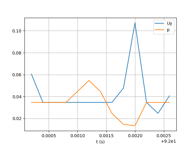
Now plots the pressure and y velocity for the first probe

import matplotlib.pyplot as plt

plt.figure()

plt.plot(timeU, u[:, 0, 1])
plt.plot(timeP, p[:, 0])

# Setting axis labels
plt.xlabel('t (s)')

# add grid and legend
plt.grid()
plt.legend(["Uy", "p"])

# show
plt.show()