Time series of postProcessing coefficient force

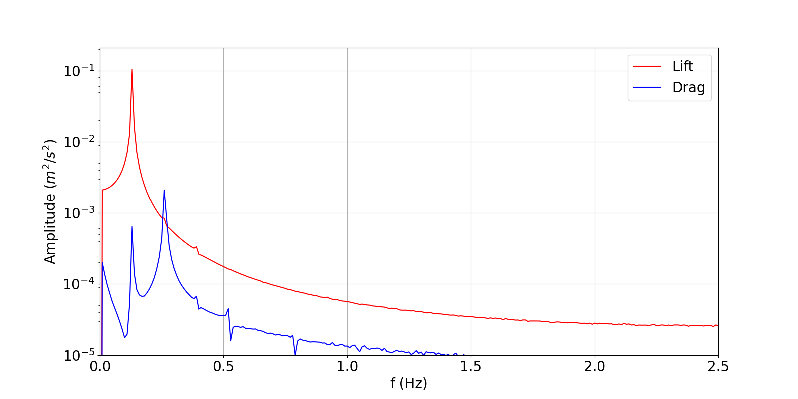
This example reads and plots one postProcessing coefficient force and compute and plot the fft of the lift coefficient force

Read the postProcessing files

Note

In this example it reads one postProcessing file for the statistically steady state of the flow around a rectangular cylinder.

from fluidfoam.readpostpro import readforce
import numpy as np

# ****************Selection of case, repository and parameters*************** #
rep = '../output_samples/'
case = 'ascii'

time = '100'                        # Simulation start time for fft
force_file_name = 'coefficient'     # Variable on which fft is applied
index_Cl = 2                        # Lift force
index_Cd = 1                        # Drag force
n0 = 0                              # Start point for the fft
nfft = 500                          # Number of point for the fft
calculdeltat = 0.01                 # Delta t used in the calculation
fftdeltat = 0.2                     # Sampling Delta t for the fft, note that Tfft = nfft * fftdeltat =< Ttot = endTime - time
timestart = 0                       # Start time for sampling from time
display_temp = True

# *************************************************************************** #

# reading Data
force = readforce(rep + case, namepatch = 'forces', time_name = time, name = force_file_name)
timevec = np.zeros(len(force))
varC = np.zeros((len(force),2))
for i in range(len(force)):
    timevec[i] = force[i,0]
    varC[i,0] = force[i,index_Cl]
    varC[i,1] = force[i,index_Cd]

# Sampling
i = 0

varCi = np.zeros((nfft,2))
vart = np.zeros(nfft)
while i < nfft:
    for k in range(2):
        varCi[i,k] = varC[int(i*fftdeltat/calculdeltat+timestart/calculdeltat), k]
    vart[i] = timevec[int(i*fftdeltat/calculdeltat+timestart/calculdeltat)]
    i += 1

# fft calculation
y1 = np.zeros((nfft,2),dtype = np.complex128)
for k in range(2):
# Division by nfft to correct the spectral amplitude
    y1[:, k] = np.fft.fft(varCi[n0:n0+nfft,k] - np.mean(varCi[n0:n0+nfft,k]))/nfft

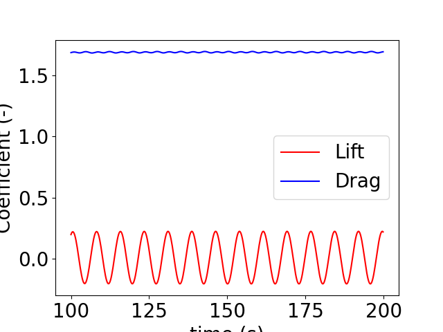
Now plots the lift and drag coefficient forces

import matplotlib.pyplot as plt

plt.rcParams.update({'font.size': 20})
# Temporal plot section
colorList = ['r', 'b']
labelList = ['Lift', 'Drag']
if display_temp:
    for k in range(2):
        plt.plot(vart[n0:n0+nfft], varCi[n0:n0+nfft,k],
             color = colorList[k], label = labelList[k])
    plt.legend(loc='best')
    plt.xlabel('time (s)')
    plt.ylabel('Coefficient (-)')
    plt.show()

# frequency plot section
f = np.arange(nfft)*1/(fftdeltat*nfft)

plt.figure(figsize=(16, 8))
for k in range(2):
    plt.semilogy(f[n0:n0+nfft], abs(y1[n0:n0+nfft,k]), color = colorList[k], label = labelList[k])

plt.axis([0.0, 1/(2*fftdeltat), 1e-5,  2*np.max(abs(y1[n0:n0+nfft]))])
plt.grid()
plt.legend(loc='upper right')
plt.xlabel(r'f (Hz)')
plt.ylabel(r'Amplitude ($m^2/s^2$)')
plt.show()

• 
•