Create vectorised visualisations of the mesh

This example shows how to use MeshVisu object to plot vectorised images of 2D planar meshes.

First create a visualisable mesh object with MeshVisu

Note

This class allows you to create a list of edges contained inside a box. This list of edges will then be ploted.

# import the class MeshVisu
from fluidfoam import MeshVisu

# path to the simulation to load
path = '../../output_samples/pipeline'

# Load mesh and create an object called myMesh
# The box by default is egal to the mesh dimension
myMesh = MeshVisu( path =  '../../output_samples/pipeline')

Reading file ../../output_samples/pipeline/constant/polyMesh/faces
Reading file ../../output_samples/pipeline/constant/polyMesh/points
Box set to mesh size:
 (minx, miny, minz) = (-0.75, -0.1, -0.001)
 (maxx, maxy, maxz) = (1.0, 0.205, 0.0)

Plot the whole mesh

import matplotlib.pyplot as plt
from  matplotlib.collections import LineCollection

# compute mesh aspect ratio:
xmin, xmax = myMesh.get_xlim()
ymin, ymax = myMesh.get_ylim()
AR = (ymax - ymin) / (xmax - xmin)

fig, ax = plt.subplots( figsize = (8,8*AR))
# create a collection with edges and print it
ln_coll = LineCollection(myMesh.get_all_edgesInBox(), linewidths = 0.25, colors = 'brown')
ax.add_collection(ln_coll, autolim=True)

# impose the dimensions of the box as the limits of the figure
ax.set_xlim(myMesh.get_xlim())
ax.set_ylim(myMesh.get_ylim())

# to avoid distorting the mesh:
ax.set_aspect('equal')

# to don't print axis:
ax.axis('off')

(-0.75, 1.0, -0.1, 0.205)

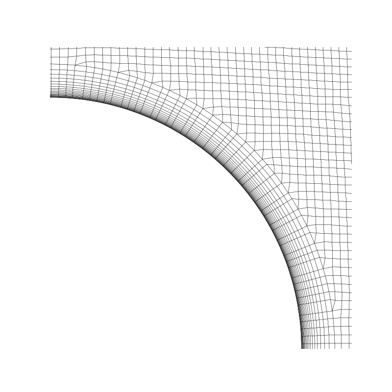
Update the box to zoom on the cylinder and save figure

myMesh.update_box(((0, 0, -1), (0.03, 0.03, 1)))

fig, ax = plt.subplots( figsize = (8,8))
# create a collection with edges and print it
ln_coll = LineCollection(myMesh.get_all_edgesInBox(), linewidths = 0.25, colors = 'black')
ax.add_collection(ln_coll, autolim=True)

# Set box dimensions as the figures's limits
ax.set_xlim(myMesh.get_xlim())
ax.set_ylim(myMesh.get_ylim())

# to avoid distorting the mesh:
ax.set_aspect('equal')

# to don't print axis:
ax.axis('off')

# to save the figure in pdf or svg format, uncomment one of the following two lines:
# plt.savefig('./myCylinderZomm.pdf', dpi=fig.dpi, transparent = True, bbox_inches = 'tight')
# plt.savefig('./myCylinderZomm.svg', dpi=fig.dpi, transparent = True, bbox_inches = 'tight')

(0.0, 0.03, 0.0, 0.03)

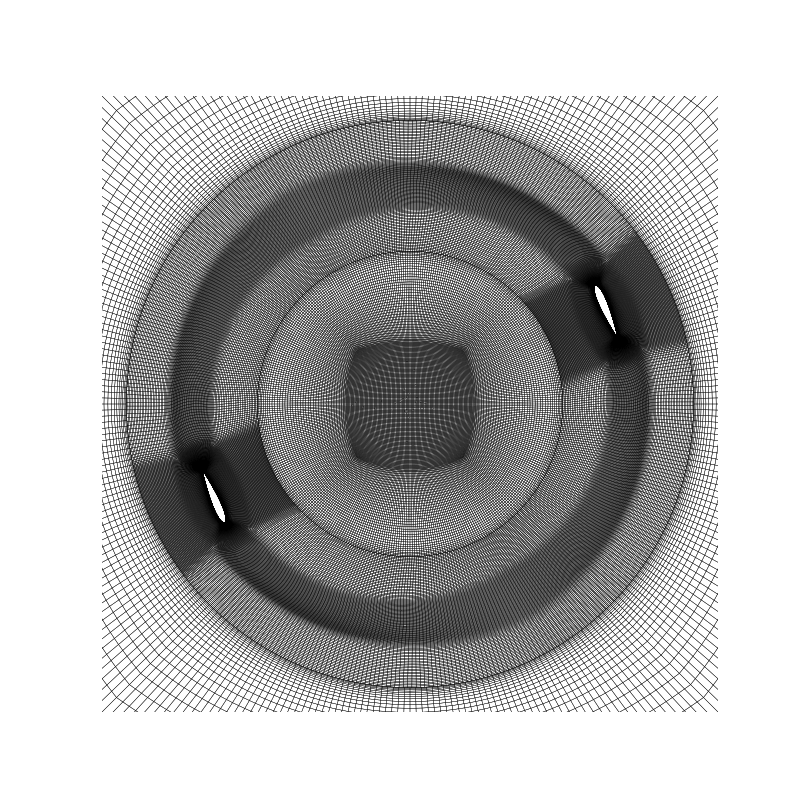
Visualisation of dynamic case in xz plane

# path to the simulation to load:
mypath =  '../../output_samples/darrieus'

# time folder for which you want to display the mesh:
mytime =  '0.1'

# plane in which the mesh is contained, either:
# 'xy': the xy-plane of outgoing normal z (default value)
# 'xz': the xz-plane of outgoing normal -y
# 'yz': the yz-plane of outgoing normal x
myplane =  'xz'

# box to zoom in on for mesh display:
mybox = ((-1.2, -1, -1.2), (1.2, 1, 1.2))

# Load mesh and create an object called myOtherMesh:
myOtherMesh = MeshVisu(path = mypath, box = mybox, time_name = mytime, plane = myplane)

# The next line sets the thumbnail for the last figure in the gallery
# sphinx_gallery_thumbnail_number = -1
fig, ax = plt.subplots( figsize = (8,8))
# create a collection with edges and print it
ln_coll = LineCollection(myOtherMesh.get_all_edgesInBox(), linewidths = 0.25, colors = 'black')
ax.add_collection(ln_coll, autolim=True)

# Set box dimensions as the figures's limits
ax.set_xlim(myOtherMesh.get_xlim())
ax.set_ylim(myOtherMesh.get_zlim())

# to avoid distorting the mesh:
ax.set_aspect('equal')

# to don't print axis:
ax.axis('off')

Reading file ../../output_samples/darrieus/constant/polyMesh/faces
Reading file ../../output_samples/darrieus/0.1/polyMesh/points

(-1.2, 1.2, -1.2, 1.2)