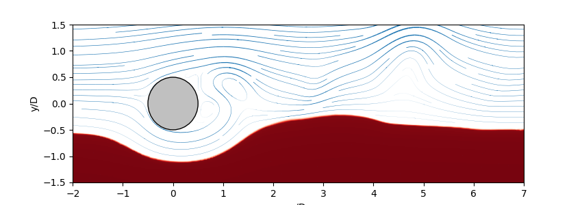
Contour and streamlines from an unstructured mesh

This example reads and plots a contour of an OpenFoam vector field from an unstructured mesh by interpolation on a structured grid

Reads the mesh

Note

It reads the mesh coordinates and stores them in variables x, y and z

# import readmesh function from fluidfoam package
from fluidfoam import readmesh

sol = '../../output_samples/pipeline/'

x, y, z = readmesh(sol)

Reading file ../../output_samples/pipeline//constant/polyMesh/owner
Reading file ../../output_samples/pipeline//constant/polyMesh/faces
Reading file ../../output_samples/pipeline//constant/polyMesh/points
Reading file ../../output_samples/pipeline//constant/polyMesh/neighbour

Reads vector and scalar field

Note

It reads vector and scalar field from an unstructured mesh and stores them in vel and alpha variables

# import readvector and readscalar functions from fluidfoam package
from fluidfoam import readvector, readscalar

timename = '25'
vel = readvector(sol, timename, 'Ub')
alpha = readscalar(sol, timename, 'alpha')

Reading file ../../output_samples/pipeline/25/Ub
Reading file ../../output_samples/pipeline/25/alpha

Interpolate the fields on a structured grid

Note

The vector and scalar fields are interpolated on a specified structured grid

import numpy as np
from scipy.interpolate import griddata

# Number of division for linear interpolation
ngridx = 500
ngridy = 180

# Interpolation grid dimensions
xinterpmin = -0.1
xinterpmax = 0.35
yinterpmin = -0.075
yinterpmax = 0.075

# Interpolation grid
xi = np.linspace(xinterpmin, xinterpmax, ngridx)
yi = np.linspace(yinterpmin, yinterpmax, ngridy)

# Structured grid creation
xinterp, yinterp = np.meshgrid(xi, yi)

# Interpolation of scalra fields and vector field components
alpha_i = griddata((x, y), alpha, (xinterp, yinterp), method='linear')
velx_i = griddata((x, y), vel[0, :], (xinterp, yinterp), method='linear')
vely_i = griddata((x, y), vel[1, :], (xinterp, yinterp), method='linear')

Plots the contour of the interpolted scalarfield alpha, streamlines and a patch

Note

The scalar field alpha reprensents the concentration of sediment in in a 2D two-phase flow simulation of erosion below a pipeline

import matplotlib.pyplot as plt

# Define plot parameters
fig = plt.figure(figsize=(8.5, 3), dpi=100)
plt.rcParams.update({'font.size': 10})
plt.xlabel('x/D')
plt.ylabel('y/D')
d = 0.05

# Add a cuircular patch representing the pipeline
circle = plt.Circle((0, 0), radius=0.5, fc='silver', zorder=10,
                    edgecolor='k')
plt.gca().add_patch(circle)

# Plots the contour of sediment concentration
levels = np.arange(0.1, 0.63, 0.001)
plt.contourf(xi/d, yi/d, alpha_i, cmap=plt.cm.Reds, levels=levels)

# Calculation of the streamline width as a function of the velociy magnitude
vel_i = np.sqrt(velx_i**2 + vely_i**2)
lw = pow(vel_i, 1.5)/vel_i.max()

# Plots the streamlines
plt.streamplot(xi/d, yi/d, velx_i, vely_i, color='C0', density=[2, 1],
               linewidth=lw, arrowsize=0.05)

<matplotlib.streamplot.StreamplotSet object at 0x7f00dfb03860>