Contour from an unstructured mesh (no interpolation)

This example reads and plots a contour of an OpenFoam vector field from an unstructured mesh by triangulation WITHOUT interpolation on a structured grid

Reads the mesh

Note

It reads the mesh coordinates and stores them in variables x, y and z

# import readmesh function from fluidfoam package
from fluidfoam import readmesh

sol = '../../output_samples/pipeline/'

x, y, z = readmesh(sol)

Reading file ../../output_samples/pipeline//constant/polyMesh/owner
Reading file ../../output_samples/pipeline//constant/polyMesh/faces
Reading file ../../output_samples/pipeline//constant/polyMesh/points
Reading file ../../output_samples/pipeline//constant/polyMesh/neighbour

Reads vector and scalar field

Note

It reads volume scalar field from an unstructured mesh and stores it

# import readvector and readscalar functions from fluidfoam package
from fluidfoam import readvector, readscalar

timename = '25'
vel = readvector(sol, timename, 'Ub')
alpha = readscalar(sol, timename, 'alpha')

Reading file ../../output_samples/pipeline/25/Ub
Reading file ../../output_samples/pipeline/25/alpha

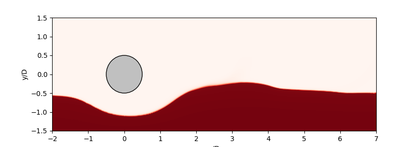
Plots the contour of the volscalarfield alpha and a patch

Note

The scalar field alpha reprensents the concentration of sediment in in a 2D two-phase flow simulation of erosion below a pipeline

import numpy as np
import matplotlib.pyplot as plt

# Define plot parameters
fig, ax = plt.subplots(figsize=(8.5, 3), dpi=100)
plt.rcParams.update({'font.size': 10})
plt.xlabel('x/D')
plt.ylabel('y/D')
d = 0.05
# Add a cuircular patch representing the pipeline
circle = plt.Circle((0, 0), radius=0.5, fc='silver', zorder=10,
                    edgecolor='k')
plt.gca().add_patch(circle)

# Plots the contour of sediment concentration
levels = np.arange(0.0, 0.63, 0.001)

plt.tricontourf(x/d, y/d, alpha, cmap=plt.cm.Reds, levels=levels)

ax.set(xlim=(-2, 7), ylim=(-1.5, 1.5))
plt.show()